
Catching Crypto Trends
Applying a Trend-Following Ensemble Approach to Bitcoin

Given the recent extreme macro uncertainty, it’s no surprise the equity market has been taking a beating. Crypto markets haven’t been immune either, though they’ve weathered the storm somewhat better than other asset classes, with promising signs of recovery popping up recently. Could it be time to revisit crypto strategies in QuantMage?

I recently stumbled upon a compelling paper by Concretum Research titled, “Catching Crypto Trends: A Tactical Approach for Bitcoin and Altcoins,” which sparked today’s deep dive. The authors test whether the classic “break-out + trailing-stop” trend-following playbook, widely effective in futures and FX, could be ported over to the fast-paced and notoriously volatile cryptocurrency market.
Trend-Following Ensemble Strategy for Bitcoin
The paper’s strategy breaks down as follows:
Signal: Donchian-channel break-outs; nine look-back horizons from 5- to 360-days.
Exit: Rolling mid-band trailing stop that never moves against the position.
Sizing: Vol-target to 25% annualized using a 90-day σ (standard deviation) with a hard cap at 2× notional.
Ensemble (“Combo”): equal-weight across the nine sub-models.
Execution: Daily rebalance, but only if volatility-driven weight drift > 20% to tame turnover.
Could we implement something similar in QuantMage? Absolutely!
QuantMage’s Aroon indicators conveniently handle Donchian-channel break-outs. However, since QuantMage doesn’t directly support the paper’s rolling mid-band trailing stop exit, I substituted it with an Ultimate Smoother crossover signal. For sizing, I used a Mixed incantation paired with a Volatility indicator. While the original paper uses nine horizons, I opted for five key horizons (20, 40, 60, 90, and 150 days) after some experimentation.
One technical adjustment is essential: the paper refers to calendar days, whereas QuantMage operates in trading days. Hence, a 90-day volatility window from the paper translates to approximately 60 trading days in QuantMage.
Here’s what I came up with:
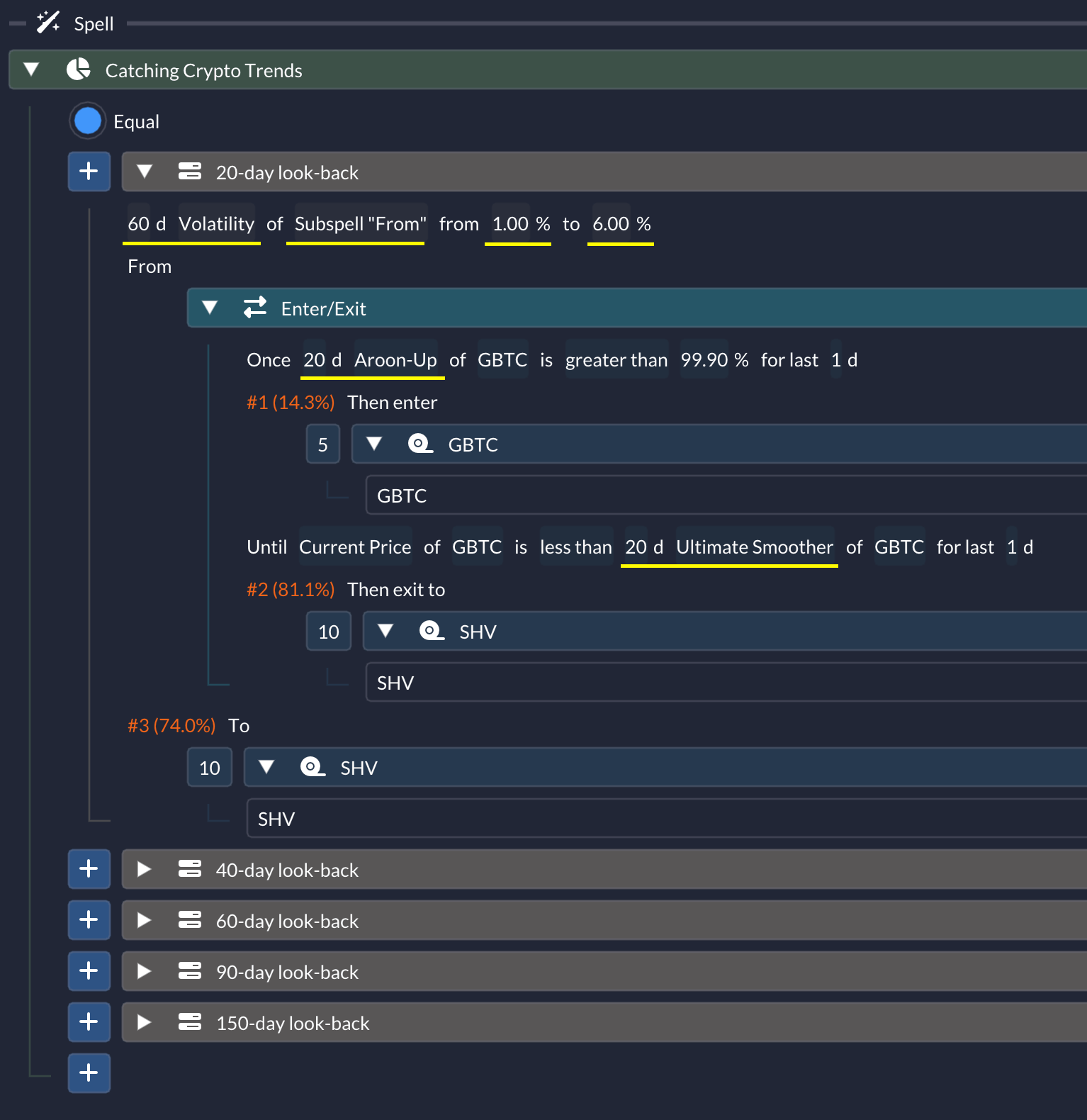
The screenshot highlights the 20-day horizon, utilizing 60-day volatility from 1% to 6%. These daily standard deviations annualize roughly between 16% to 95%, bracketing the 25% annualized volatility threshold used in the original paper for position sizing. If the trend-following sub-strategy’s volatility falls below 16%, the portfolio shifts entirely to the sub-strategy that invests in GBTC (a Bitcoin ETF since Jan 2024). Conversely, if the volatility exceeds 95%, it goes fully defensive into SHV, a short-term treasury bond ETF. For volatility between these thresholds, the allocation smoothly blends the sub-strategy and SHV.
A notable divergence from the original paper is in the sizing logic. The paper targets Bitcoin’s volatility directly, whereas my implementation measures the volatility of the sub-strategy performance. This seemingly minor difference notably influenced historical performance. Another important discrepancy is the use of GBTC, which had a notable tracking error before its conversion to a Bitcoin ETF in January 2024, potentially introducing additional noise into the strategy’s risk and return profile.
Backtesting Results
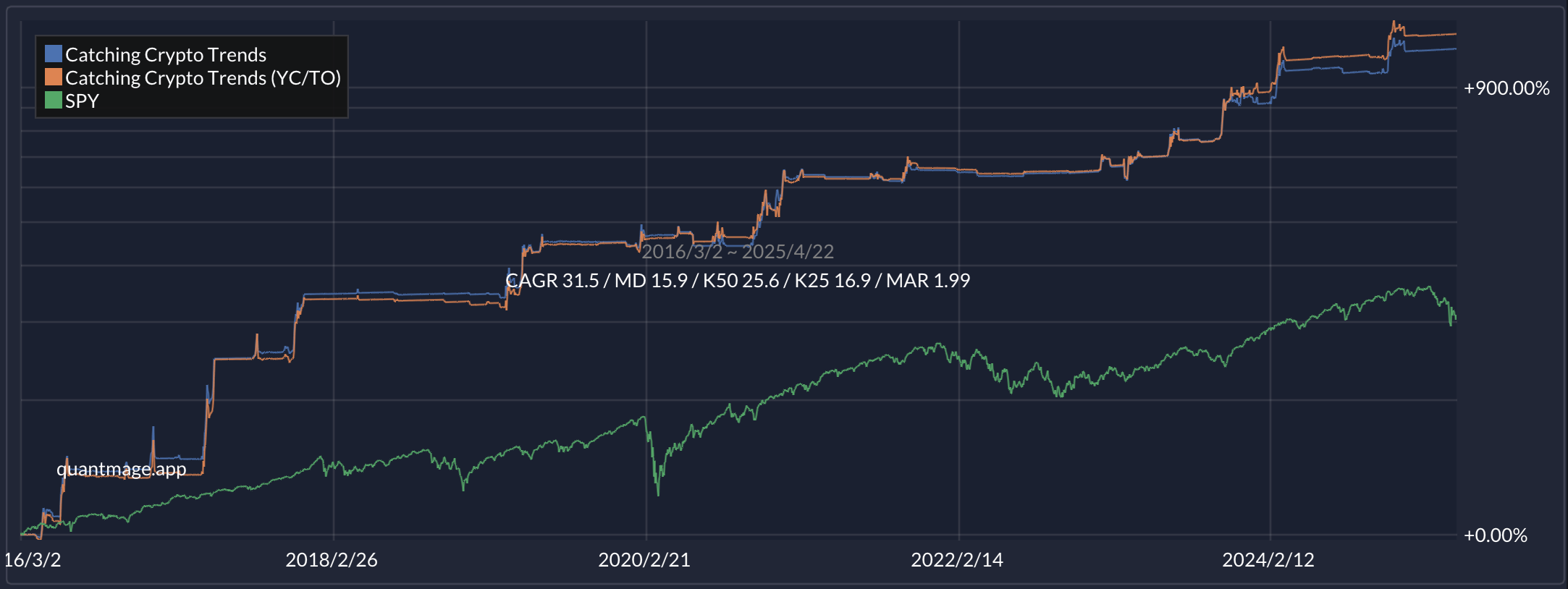
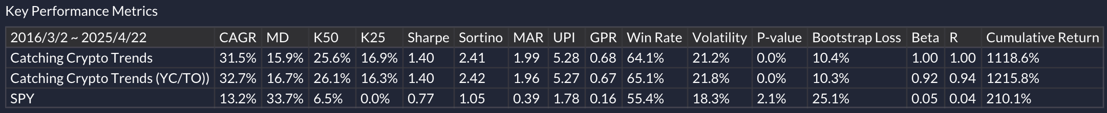
The strategy showed an impressive compound annual growth rate (CAGR) of 31.5% with a maximum drawdown of 15.9% over a nine-year backtest, resulting in a strong Sharpe ratio of 1.4. Although this doesn’t match Bitcoin’s raw returns, the results are exceptional on a risk-adjusted basis—closely aligning with the paper’s reported performance (CAGR 30%, Max Drawdown 19%, Sharpe 1.58).
Interestingly, substituting the defensive asset SHV with a gold ETF like IAU generated an equally intriguing historical performance. You can do such a swapping in one go with QuantMage’s Adhoc Synchronized Editing. Curious? Try the strategy yourself here.
🚨 Disclaimer: This content is informational only and not investment advice. Always do your due diligence and consider consulting a financial advisor before making investment decisions.
Bottom Line
What strikes me most is how this strategy achieves a relatively smooth equity curve using a highly volatile underlying asset like Bitcoin. I highly recommend checking out the original paper for deeper insights.
What’s your perspective? Do you believe this approach can maintain its historical performance, or has Bitcoin evolved too significantly? Does this inspire you to explore similar trend-following ensembles or volatility-driven sizing strategies with other asset classes?
I’m eager to hear your thoughts! 💭
It's interesting that you did this, I recently backtested a trend-following approach with bitcoin/GBTC as well after reading about the approaches that turtle traders used. It seemed to me that the approach worked much better in early years and has kind of settled down in the last few years. Maybe bitcoin is morphing into something more equity-like. I think it's worth following up on though.